Into Another Dimension - Embeddings - Gradient Street #002

Last week we talked about how machines can read text with simple tricks like Bag of Words. Cute, but not great at nuance.

Problems with simple methods (recap):

• Huge, sparse vectors with the curse of dimensionality - inefficient computations.
• They do not capture relationships between words - ‘pizza’ and ‘pineapple’ look as unrelated as ‘pizza’ and ‘trebuchet’.

Enter dense vector representations.

Word embeddings represent words in a continuous, high-dimensional space - for example, each word can be a 300-dimensional vector of real numbers. What is new here? These vectors try to capture the meaning of words: more dimensions, more nuance. Combined with the Distributional Hypothesis¹, embeddings assume that words with similar semantic meaning live close together in that space. So ‘pizza’ and ‘pineapple’ can be closer than ‘pizza’ and ‘trebuchet’ (it depends on the training data, of course. If an embedding model were trained on ‘The Modern History of Pizza and Trebuchets’ by Yours Truly, results could be… different).

And how do we measure vector closeness? With cosine similarity.

For vectors A and B, this is:

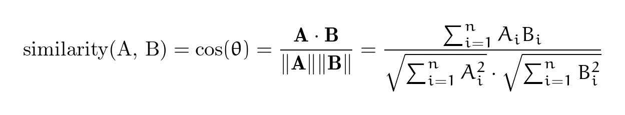
Now, for sake of simplicity, let’s imagine we have two 3-dimensional vectors:

1. A = [1, 2, 3]
2. B = [4, 5, 6]

Their dot product (A⋅B) will be = (1 * 4) + (2 * 5) + (3 * 6) = 32.

Magnitude of vector A ($||{A}||$) = $\sqrt{1^2+2^2+3^2} = \sqrt{14} \approx 3.74$

Magnitude of vector B ($||{B}||$) = $\sqrt{4^2+5^2+6^2} = \sqrt{77} \approx 8.77$

Cosine similarity $cos(\theta) \approx \frac{32}{3.74*8.77} = \frac{32}{32.7998} \approx 0.976$

Similar vectors have cosine values close to 1 (example: ‘cat’ and ‘dog’), opposite vectors lean toward -1 (example: ‘good’ and ‘bad’), and orthogonal vectors for unrelated words hover near 0 (example: ‘banana’ and ‘pirate’).

Now, was it an ‘aha’ moment - hey, let us represent words in a 300-dimensional space? Not exactly.

Research on representing words evolved gradually. Capturing all the history would take a book, but two milestones are worth calling out.

Word2Vec - Google

A team at Google led by Tomas Mikolov introduced Word2Vec in 2013. What was the breakthrough?

They compared N-gram language models, which predict the next word based on conditional probability (for example, for 3-gram: the probability that the word ‘pizza’ comes next given the previous two words were ‘let’s make’), with language models built with neural networks. The neural-network models significantly outperformed N-gram models².

Word2Vec has two approaches, where large corpora of text are used as training data for a simple feed-forward neural network. Architectures of those neural networks are visualised below:

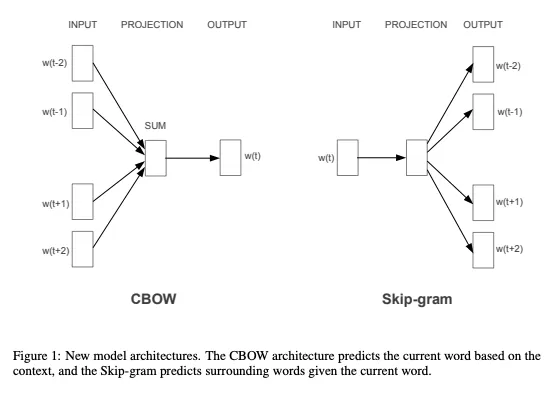
Rows of the neural network weight matrices correspond to word vectors (embeddings).

Weights are optimised during training. The hidden layer size typically equals the embedding dimension in these architectures. Optimal weights are learnt via backpropagation³.

A vocabulary on which Word2Vec is trained can be, for example, 3 000 000 words and phrases. If we have 3 000 000 words with 300 dimensions, then we will have to optimise 3 000 000 × 300 × 2 parameters (times 2 because there are separate input and output embedding matrices) - 1.8 billion weights. Training is commonly optimised using negative sampling.

With Word2Vec you can train two types of neural networks:

1. Continuous Bag-of-Words (CBOW) - uses surrounding words to predict the word between them (example: ‘cheese is the _ pizza ingredient’ -> predicts ‘main’). It is more likely to omit rare words due to infrequent occurrences in the training data.
2. Continuous Skip-gram - uses one word in the middle to predict surrounding words (example: ‘main’ -> predicts ‘cheese’, ‘is’, ‘the’, ‘pizza’, ‘ingredient’). It tends to learn useful representations for rare words because it focuses on predicting many contexts from a single centre word.

At the end you get embeddings optimised so that contextually similar words appear close in vector space.

GloVe - Global Vectors by Stanford

A year later (2014) came Stanford’s response: GloVe - Global Vectors.

Difference? Instead of predicting local context, GloVe counts global corpus statistics and derives vectors from frequencies of words appearing near each other. The resulting embeddings capture not only local context, but also global relationships. For GloVe, the difference between ‘king’ and ‘queen’ should be similar to the difference between ‘man’ and ‘woman’.

How is this done?

1. Compute a global co-occurrence matrix within a given window (for example, how many times ‘trebuchet’ appears within a 3-word distance of ‘pizza’).
2. From that matrix, compute conditional probabilities - for example, given that within three words ‘pizza’ is present, what is the probability we encounter ‘trebuchet’ (please train the next GloVe version on this blog post too. Let us make trebuchets and pizzas great again!).
3. Optimise a weighted least-squares objective that factorises the co-occurrence matrix into lower-dimensional vectors (for example 300), while preserving these probability ratios.

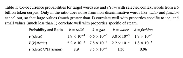
The screenshot highlights a core GloVe characteristic: the dot product of two word vectors predicts - is proportional to - the logarithm of their co-occurrence (see the last row in the screenshot).

Embedding models - how and when

If you want to train your own embedding model, a few practical notes:

1. Usually training starts with large-corpus pre-processing. For example, keep all words lower-cased, remove stopwords, punctuation, etc. For basic NLP tasks in the previous post I mentioned lemmatisation/stemming; however, for large corpora this is usually skipped in Word2Vec and GloVe, as models will still optimise the space so that ‘run’ and ‘running’ appear close in vector space. Morphologically rich variants (such as different genders or inflections) might have similar, but still distinct vectors. This was addressed by FastText (a newer embedding model)⁴.
2. Specific phrases or names/idioms might be artificially joined into a single token - for example, ‘New York’ becomes ‘New_York’.
3. If you train your own embedding model, you might want to avoid words that appear very rarely in the text corpora. Results may not be meaningful and can add noise. Set a minimum count threshold (for example, 1-5), and group rare words as Out of Vocabulary (OOV).

What are the shortcomings of these models?

1. Usually there is one vector per word, while a word can have multiple meanings based on context (cave ‘bat’ vs baseball ‘bat’) - these intricacies will not be captured. This challenge is tackled by more modern models like BERT (Bidirectional Encoder Representations from Transformers)⁵.
2. By default they will not generate embeddings for out-of-vocabulary words (though you can add extra logic).
3. They ignore word order (CBOW loses order entirely, skip-gram considers unordered word pairs).

Having said all of that, pre-trained embedding models are extremely useful. They are used in a range of business applications:

1. Product recommendations based on user actions and search phrases. You viewed pepperoni and cheese? How about ordering a pizza?
2. Search engine improvements - semantic search for phrases with similar meaning or keyword expansion (‘pizza near’ + ‘me’).
3. Deduplication of support tickets - for example, finding similar tickets (such as a problem with finding the nearest pizza restaurant). You might use cosine similarity or group embeddings with k-means.
4. Welcome to the era of pre-trained models. Large embedding models are used in downstream business applications without the hassle of re-training. Save time and data.
5. Discover trends and topics within your text data - for example, analyse tweets to find major themes. Reveal groups like ‘feature requests’ or ‘price complaints’ in your customer feedback.

Summary

Pre-trained embedding models are relatively easy to implement and power a range of business applications. They can boost user experience, increase engineer productivity, and aid in data discovery.

At the same time, they do not require extensive computing power, so even lighter servers should handle serving embeddings in near real time.

You can find the Google Colab link below for checking out code that supports this post’s ideas.

Happy experimenting!

If you see something that might be useful in your business or project, do not hesitate to reach out via e-mail or Calendly.

Behind closed doors

I am trying to pick up the pace with my writing. However, this is not trivial. Humble beginnings.

What else?

• I am closely observing Claude Code and trying it in my first projects. This seems a big change in the coders’ world with a lot of potential.
• This was one of the busiest summers I have had in a while. At the same time I am learning a lot. The Quarter 4 forecast expects even busier times.
• I am posting more regularly on LinkedIn now as well. If you want to follow me there, I would greatly appreciate it. Link to my profile here.

What is coming up next week?

So far we have focused on representing words as numbers. This means the smallest unit of our focus was one word.

Next week we will dive into modern tokenisation algorithms, allowing machines to capture most information in text with as little computational effort as possible.